5  Non-linear Regression

Required packages

library(tidyverse)  # tidy and wrangle data
library(broom)      # create tidy tables for statistical objects
library(effectsize) # calculate effect size
library(kableExtra) # create tidy tables
library(faux)       # simulate factorial data
library(tibble)     # create tables
library(pscl)

5.1 Non-Linear Regression

Linear regression does not work for:

• binary outcomes: For example, predicting a disease (yes/no) based on the age, sex, smoking and blood pressure. Alternative: logistic regression

• discrete outcomes: For example, classify severity as low, medium or high. Alternative: ordinal logistic regression.

• count outcomes: For example, number of hospital visits, number of cigarettes smoked per day. Alternative: poisson regression or negative binomial regression

Generalized linear models, which extend the linear regression model to work with binary, discrete and count outcomes and other data that cannot be fit well with normally distributed errors.

par(mfrow = c(2, 2))
hist1 <- hist(rnorm(4000, 0, 1), main = "Normal distirbution", xlab = NULL)
hist2 <- hist(rbinom(4000, 1, 0.05), main = "Binomial distirbution", xlab = NULL)
hist3 <- hist(rgamma(4000, 1, 100), main = "Gamma distirbution", xlab = NULL)
hist4 <- hist(rpois(4000, 0.5), main = "Poisson distirbution", xlab = NULL)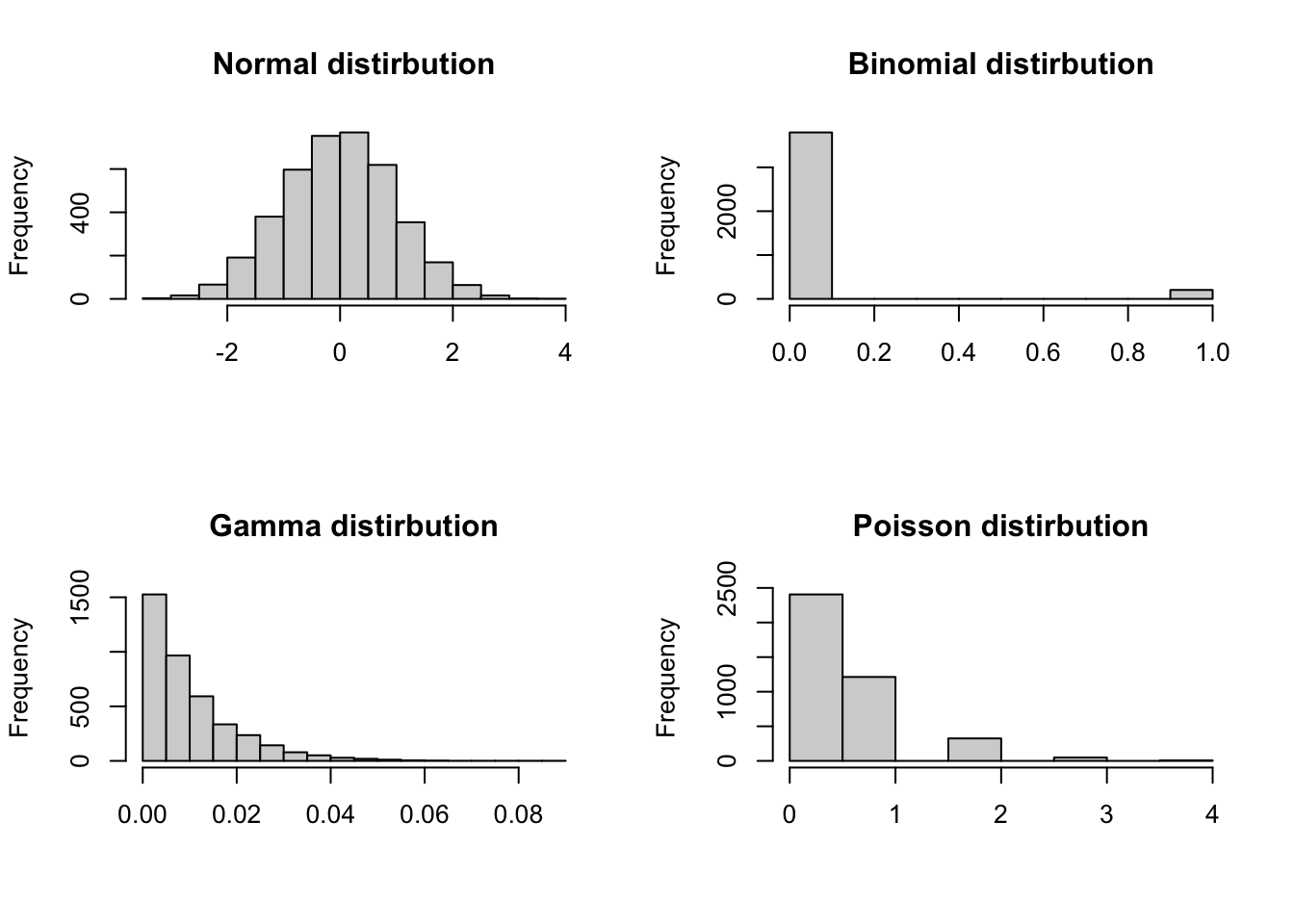

Types of distirbutions

Distribution	Description
Normal	Standard linear regression is useful when data follows a bell-shaped distribution.
Binomial	Binary logisitic regression.Useful when the response is binary (e.g., yes/no).
Gamma	Gamma regression is useful when data is highly positively skewed.
Poisson	Poisson regression is useful for count data.

5.1.1 Logistic regression

In linear regression, the outcome is a continuous variable, meaning that it can take on a range of numerical values. In contrast, logistic regression is used when the outcome is binary-that is, a categorical variable with exactly two possible values, such as “yes” or “nor”, “success” or “failure”, or “disease” or “no disease”. To model binary data, we need to add two features to the base model y = b0+ b1x1:

• a nonlinear transformation that bounds the output between 0 and 1 (unlike y = b0+ b1x1, which is continuous), and

• a model that treats the resulting numbers as probabilities and maps them into random binary outcomes.

Logistic regression models the probability of one of these outcomes occurring as a function of one or more predictor variables. For example, logistic regression can be used to model the relationship between between heart coronary disease (yes or no) and predictors such as age and blood pressure. Similarly, it can be used to model the probability of a student dropping out of school (yes or no) based socioeconomic factors.

The model of a logistic regression

In logistic regression, the model estimates the log-odds of the binary outcome y as a linear function of predictors:

\[ log(\frac{P(Y = 1)}{P(Y = 0)}) = b_0 + b_{1}x_{1} + b_{2}x_{2} + ... + b_{p}x_{p} \]

• b0: the intercept is log-odds of the outcome when all predictors are equal to zero. Exponentiating b0 gives the odds of the outcome when all predictors are equal to 0.

• If x is a continuous predictor the regression coefficient b represents the change in the log-odds of the outcome per one-unit increase in x, holding all other predictors constant. Equivalently, exp(b) is the odds ratio (OR) for a one-unit increase in x.

• If x is a categorical predictor (with k levels) is represented using dummy variables, comparing each level to a reference category. The coefficient b for a given level represents the difference in log-odds of the outcome between that category and the reference category, again holding other variables constant. Equivalently, exp(b) is the odds ratio comparing that level to the reference level.

5.1.1.1 Why not to use a linear regression when outcome is binary

First let’s simulate data where disease is a binary outcome and cholesterol is a continuous predictor.

# for reproducibility
set.seed(050990)

# create a binomial variable
disease <- rbinom(500, 1, 0.5)

# create a continuous predictor
cholesterol <- ifelse(disease == 1, rnorm(500, 220, 10), rnorm(500, 190, 10))

# create a data set
disease_df <- data.frame(disease = disease, cholesterol = cholesterol)

head(disease_df, 5)

  disease cholesterol
1       1    207.6714
2       1    254.9519
3       1    235.0051
4       1    193.6956
5       0    193.1898

Now let’s illustrate the relationship between disease and cholesterol.

ggplot(disease_df, aes(y = disease, x = cholesterol)) +
  geom_point() +
  ylim(c(0, 1)) +
  xlim(c(140, 300)) +
  geom_smooth(method = lm, se = FALSE, colour = "red")

`geom_smooth()` using formula = 'y ~ x'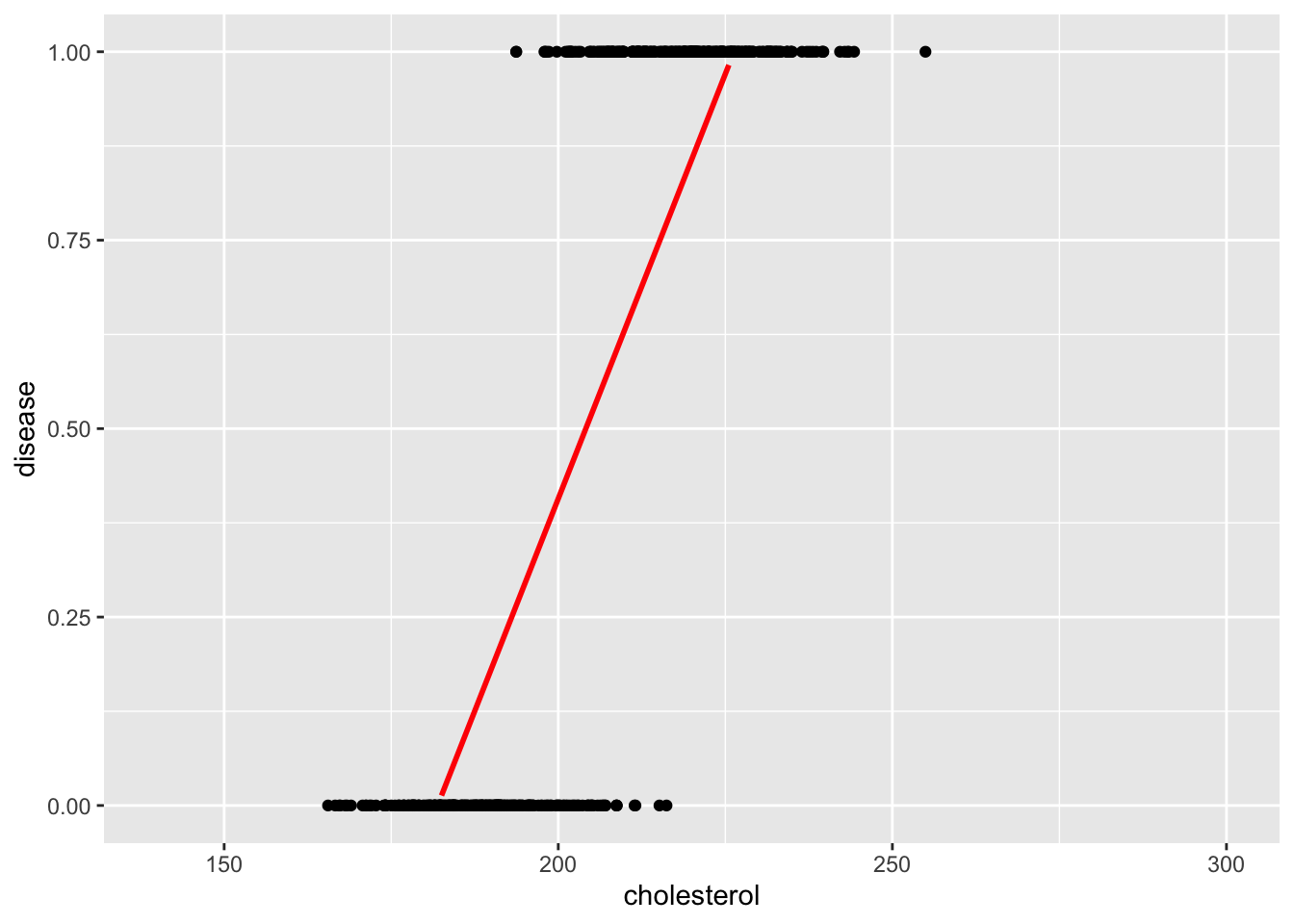

The straight line fitted using a linear model poorly fits the data. However, the red S-shaped curve better reflects the probability structure of binary data.

ggplot(disease_df, aes(y = disease, x = cholesterol)) +
  geom_point() +
  ylim(c(0, 1)) +
  xlim(c(140, 300)) +
  geom_smooth(method = glm, method.args= list(family = "binomial"), se = FALSE)

`geom_smooth()` using formula = 'y ~ x'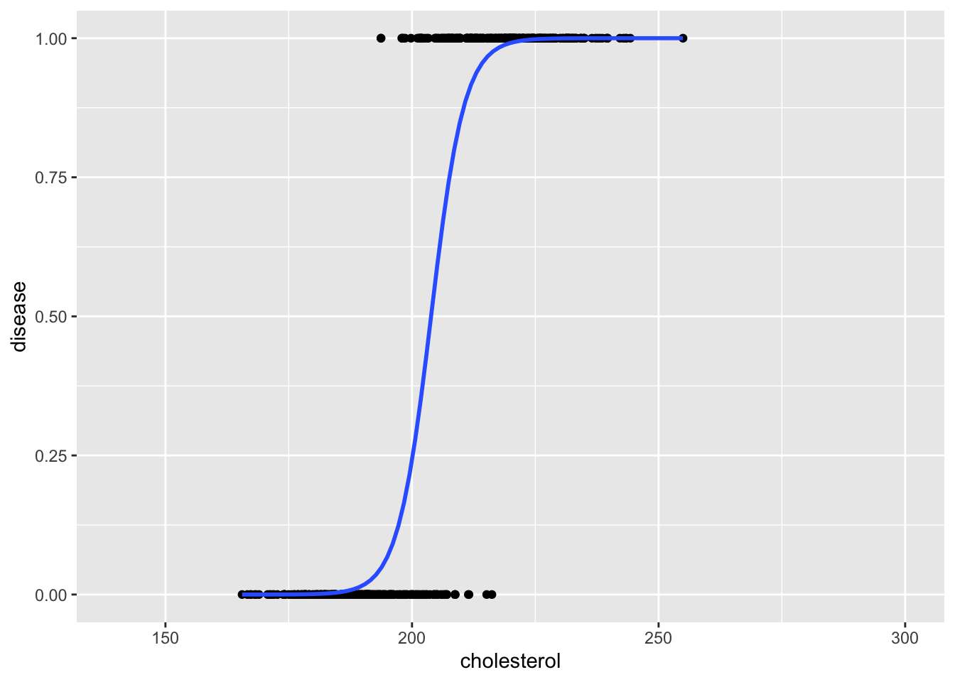

Another key problem when using a linear regression model for binary outcomes is that the estimated values (interpreted as probabilities) can fall outside the range 0-1.

linear_model <- lm(disease ~ cholesterol, disease_df)

tidy(linear_model)

# A tibble: 2 × 5
  term        estimate std.error statistic   p.value
  <chr>          <dbl>     <dbl>     <dbl>     <dbl>
1 (Intercept)  -4.10    0.136        -30.0 6.28e-114
2 cholesterol   0.0225  0.000667      33.8 4.79e-131

For example, when cholesterol is 0, the linear model estimates that the probability of disease is -4.1 - which is not a valid probability. In contrast, logistic regression constrains the estimated values within the range [0, 1] making it appropriate for classification tasks. In R we can fit a logistic linear regression using glm(family = binomial).

Note

Contrast with Linear Regression:

• Linear regression minimizes the vertical distance (squared errors) between observed data points and the fitted line.

• Logistic regression maximizes the likelihood - the joint probability of the observed outcome given the model’s predicted probabilities (i.e., the parameter estimates are those values which maximize the likelihood of the data which have been observed).

5.1.1.2 Interpreting logistic regression coefficients

To interpret the logistic regression output, we need to transform the coefficients from the log-odds scale to OR and probabilities.

1- Fit a logistic simple model:

# fit a logistic simple model
logistic_model1 <- glm(disease ~ cholesterol, family = binomial, data = disease_df)
logistic_model1$coefficients

(Intercept) cholesterol 
-60.2681245   0.2956278 

As it appears now, (Intercept) and cholesterol represent the log-odds of disease.

2- Convert coefficients to Odds Ratios using exp():

or_b1 <- exp(coef(logistic_model1)[[2]])
or_b1

[1] 1.34397

Each 1-unit increase in cholesterol is associated with 1.34x higher odds of having the disease.

3- Estimate the probability of disease for a given cholesterol level

intercept <- coef(logistic_model1)[[1]]
slope <- coef(logistic_model1)[[2]]

# Cholesterol value
cholesterol <- 200

# Compute log-odds
log_odds <- intercept + slope*cholesterol

#Convert to probability of disease
prob <- 1 / (1 + exp(-log_odds))
prob

[1] 0.2418507

Alternatively, we can use predict(type = response) to calculate the probability of disease`

# Create a data frame with new values
new_data <- data.frame(cholesterol = c(200, 250))

# Use predict(type = "response") to estimate probabilities for any given value 
predict(logistic_model1, new_data, type = "response")

        1         2 
0.2418507 0.9999988 

5.1.1.3 About odds and odds ratios

5.1.1.3.1 Odds

The odds of an event are the ratio of how likely the event is to occur and how likely it is to not occur. Odds express likelihood relative to non-occurrence. Odds are calculated as:

\[ \frac {p}{(1-p)} \]where p is the probability of an event happening, and 1-p is the probability that the event does not happen. For example, if an event has a probability of 0.8, then the odds are:

\[ \frac {0.8}{(1-0.8)} = \frac {0.8}{0.2} = 4 \]

which is read as “4 to 1”.

When the probability is greater than 50% (0.5), the odds are always greater than 1. When the probability of an event are is smaller than 50%, the odds are smaller than 1. When the probability is 50%, the odds equal 1.

5.1.1.3.2 Odds ratios

An odds ratio (OR) compares the odds of an event occurring in one group to the odds of the same event occuring in another group. It quantifies how much more (or less) likely the event is in one group compared to the other. For example, suppose the probability of disease is 0.25 for patients with high cholesterol and 0.15 for patients with adequate levels. The OR is, therefore, calculated as:

or <- (0.25 / (1-0.25)) / (0.15 / (1-0.15))
or

[1] 1.888889

An OR of 1.89 implies that the first group has 89% greater odds of developing the disease than the second group.

5.1.1.3.3 An example using a frequency table

Exposure Status	Disease = Yes	Disease = No	Total
Smoker	30	70	100
Non-smoker	10	90	100

• Odds of disease among exposed:

  \[ \frac {30}{70} = 0.43 \]

• Odds of disease among unexposed:

  \[ \frac {10}{90} = 0.11 \]

• Odds Ratio:

  \[ \frac {0.43} {0.11} = 3.86 \]

Interpretation:

• The odds of disease in the exposed group are 0.43

• The odds of disease in the unexposed group are 0.11

• The odd ratio is 3.86, meaning the exposed group has 3.86 times higher odds of developing the disease compared to the unexposed group.

5.1.1.4 Multiple logistic regression

Just like in the linear regression, we can fit more than one predictor.

5.1.1.4.1 Model with one continuous predictor and one categorical predictor

Let’s create a second predictor of disease (i.e., smoking):

# for reproducibility
set.seed(050990)

# create a binary predictor (smoking)
smoking <- ifelse(disease == 1, rbinom(500, 1, 0.7), rbinom(500, 1, 0.10))

# add the new variable to the disease_df data set
disease_df$smoking <- as.factor(smoking)

head(disease_df, 5)

  disease cholesterol smoking
1       1    207.6714       0
2       1    254.9519       0
3       1    235.0051       1
4       1    193.6956       0
5       0    193.1898       1

Let’s fit model with both cholesterol and smoking as predictors of disease.

logistic_model2 <- glm(disease ~ cholesterol + smoking, family = binomial, disease_df)

tidy(logistic_model2)

# A tibble: 3 × 5
  term        estimate std.error statistic  p.value
  <chr>          <dbl>     <dbl>     <dbl>    <dbl>
1 (Intercept)  -59.9      6.44       -9.30 1.44e-20
2 cholesterol    0.292    0.0315      9.27 1.87e-20
3 smoking1       1.86     0.551       3.37 7.55e- 4

Rather than using the exp() function to convert log-odds coefficient of each single predictor to an OR like this:

exp(coef(logistic_model2)[[2]])

[1] 1.33875

We can use tidy() in the broom package with the argument exponentitate = TRUE to obtain the ORs for all predictors at once

res <- tidy(logistic_model2, exponentiate = TRUE)
res

# A tibble: 3 × 5
  term        estimate std.error statistic  p.value
  <chr>          <dbl>     <dbl>     <dbl>    <dbl>
1 (Intercept) 9.93e-27    6.44       -9.30 1.44e-20
2 cholesterol 1.34e+ 0    0.0315      9.27 1.87e-20
3 smoking1    6.41e+ 0    0.551       3.37 7.55e- 4

We can interpret these coefficients as follows:

• cholesterol: For each 1-unit increase, the odds of disease increase by 34%. This increase is statistically significant.

• smoking1: being a smoker (smoking1 = 1) increases the odds of disease by 541 % compared to a non-smoker. This increase is statistically significant.

We can also obtain the confidence intervals (CIs) for the odds ratios by exponentiating the confidence intervals of the model coefficients:

# subset rows 2 and 3 since these correspond to the predictors
exp(confint(logistic_model2))[2:3,]

Waiting for profiling to be done...

               2.5 %    97.5 %
cholesterol 1.266617  1.434272
smoking1    2.274929 20.022067

Alternatively, we can use tidy() in the broom package with the argument conf.int = TRUE (along with exponentiate = TRUE) to get the odds ratios and their confidence intervals all at once:

tidy(logistic_model2, 
     exponentiate = TRUE,
     conf.int = TRUE)

# A tibble: 3 × 7
  term        estimate std.error statistic  p.value conf.low conf.high
  <chr>          <dbl>     <dbl>     <dbl>    <dbl>    <dbl>     <dbl>
1 (Intercept) 9.93e-27    6.44       -9.30 1.44e-20 7.43e-33  8.29e-22
2 cholesterol 1.34e+ 0    0.0315      9.27 1.87e-20 1.27e+ 0  1.43e+ 0
3 smoking1    6.41e+ 0    0.551       3.37 7.55e- 4 2.27e+ 0  2.00e+ 1

Now let’s simulate the probability of disease:

# Get the levels from the original data
levels(disease_df$smoking)

[1] "0" "1"

# Create new values 
new_data <- data.frame(
  cholesterol = c(50, 50, 200, 200),
  smoking = factor(rep(c(0,1), 2), levels = levels(disease_df$smoking))
)

# Add predictions
predicted_prob <- predict(logistic_model2, new_data, type = "response")

# Store both numeric and pretty-formatted percentages
new_data$probability <- round(predicted_prob * 100, 2)  

new_data

  cholesterol smoking probability
1          50       0        0.00
2          50       1        0.00
3         200       0       17.84
4         200       1       58.19

5.1.1.4.2 Model with an interaction between two predictors

In this section, we analyze a dataset containing health records of patients to predict a binary outcome: whether a patient suffers from diabetes (diabetes: yes = 1 / no = 0).

The goal is to explore how various physiological indicators—such as body mass index, blood pressure, and glucose levels—are associated with the likelihood of diabetes.

Load and clean the data:

data <- read.csv("https://raw.githubusercontent.com/plotly/datasets/master/diabetes.csv")

colnames(data)<-tolower(colnames(data))

data$outcome<-as.factor(data$outcome) 

head(data, 5)

  pregnancies glucose bloodpressure skinthickness insulin  bmi
1           6     148            72            35       0 33.6
2           1      85            66            29       0 26.6
3           8     183            64             0       0 23.3
4           1      89            66            23      94 28.1
5           0     137            40            35     168 43.1
  diabetespedigreefunction age outcome
1                    0.627  50       1
2                    0.351  31       0
3                    0.672  32       1
4                    0.167  21       0
5                    2.288  33       1

Fit a regression model with an interaction term between

# Fit a multiple regression logistic model
logistic_model3 <- glm(outcome ~ age + glucose*bmi, data = data, family="binomial")

# Use tidy() to make it more readable
res <- tidy(logistic_model3, exponentiate = TRUE)

# Make estimates and p-values more interpretable
res <- res |> 
  mutate(estimate_round = round(estimate, 2),
         p_value = round(p.value, 2)) |> 
  select(term, estimate_round, std.error, statistic, p_value)

res

# A tibble: 5 × 5
  term        estimate_round std.error statistic p_value
  <chr>                <dbl>     <dbl>     <dbl>   <dbl>
1 (Intercept)           0     2.25        -4.50     0   
2 age                   1.03  0.00770      3.81     0   
3 glucose               1.05  0.0177       2.64     0.01
4 bmi                   1.14  0.0653       2.04     0.04
5 glucose:bmi           1     0.000508    -0.815    0.42

Interpretation:

• age: Every 1-year increase in age increases the odds of diabetes by 3%. This increase is statistically significant.

• glucose: Every 1-unit increase in glucose increases the odds of diabetes by 5%. This increase is statistically significant.

• bmi: Every 1-unit increase in body mass index increases the odds of diabetes by 14%. This increase is statistically significant.

• glucos:bmi: The effect of glucose on the odds of diabetes does not increase as bmi increases. The interaction effect is not statistically significant.

5.1.1.5 Centering

glm(outcome ~ glucose + bloodpressure, data = data, family="binomial") |> 
tidy(exponentiate = TRUE)

# A tibble: 3 × 5
  term          estimate std.error statistic  p.value
  <chr>            <dbl>     <dbl>     <dbl>    <dbl>
1 (Intercept)    0.00518   0.486     -10.8   2.57e-27
2 glucose        1.04      0.00329    11.6   7.22e-31
3 bloodpressure  0.998     0.00443    -0.354 7.23e- 1

(intercept) represents the odds of diabetes when all other variables are 0. However, interpreting (intercept) when glucose = 0 and bloodpressure = 0 is not meaningful as it is physiologically impossible. We can make (intercept) more interpretable by centering the predictors.

# Center the predictors
data$glucose_centered <- data$glucose - mean(data$glucose)
data$bloodpressure_centered <- data$bloodpressure - mean(data$bloodpressure)

# Refit the logistic regression model with the centered predictors
res <- glm(outcome ~ glucose_centered + bloodpressure_centered, 
           data = data, family="binomial") |> 
  tidy(exponentiate = TRUE)

res

# A tibble: 3 × 5
  term                   estimate std.error statistic  p.value
  <chr>                     <dbl>     <dbl>     <dbl>    <dbl>
1 (Intercept)               0.462   0.0883     -8.74  2.40e-18
2 glucose_centered          1.04    0.00329    11.6   7.22e-31
3 bloodpressure_centered    0.998   0.00443    -0.354 7.23e- 1

Interpretation:

• (intercept): When glucose and bloodpressure are at their average levels, the odds of diabtes are 0.46.

• glucose_centered: Every 1-unit increase in glucose significantly increases the odds of diabetes by 4%.

• bloodpressure: Every 1-unit increase in blood pressure decreases the odds of diabetes by -0.16%. However, this is not statistically significant.

5.1.1.6 Model fit

Suppose we want to compare whether adding bmi to a simpler model increases the fit of the model:

Simpler model

model1 <- glm(outcome ~ glucose + bloodpressure + insulin, 
             data = data, family="binomial") 

summary(model1)

Call:
glm(formula = outcome ~ glucose + bloodpressure + insulin, family = "binomial", 
    data = data)

Coefficients:
                Estimate Std. Error z value Pr(>|z|)    
(Intercept)   -5.3381664  0.4943004 -10.799   <2e-16 ***
glucose        0.0390197  0.0034669  11.255   <2e-16 ***
bloodpressure -0.0013534  0.0044319  -0.305    0.760    
insulin       -0.0007271  0.0007565  -0.961    0.336    
---
Signif. codes:  0 '***' 0.001 '**' 0.01 '*' 0.05 '.' 0.1 ' ' 1

(Dispersion parameter for binomial family taken to be 1)

    Null deviance: 993.48  on 767  degrees of freedom
Residual deviance: 807.68  on 764  degrees of freedom
AIC: 815.68

Number of Fisher Scoring iterations: 4

Model with bmi

model2 <- glm(outcome ~ glucose + bloodpressure + insulin + bmi, 
             data = data, family="binomial")

summary(model2)

Call:
glm(formula = outcome ~ glucose + bloodpressure + insulin + bmi, 
    family = "binomial", data = data)

Coefficients:
               Estimate Std. Error z value Pr(>|z|)    
(Intercept)   -7.433886   0.657526 -11.306  < 2e-16 ***
glucose        0.037708   0.003531  10.679  < 2e-16 ***
bloodpressure -0.007430   0.004907  -1.514   0.1300    
insulin       -0.001493   0.000785  -1.902   0.0572 .  
bmi            0.083887   0.013880   6.044  1.5e-09 ***
---
Signif. codes:  0 '***' 0.001 '**' 0.01 '*' 0.05 '.' 0.1 ' ' 1

(Dispersion parameter for binomial family taken to be 1)

    Null deviance: 993.48  on 767  degrees of freedom
Residual deviance: 765.48  on 763  degrees of freedom
AIC: 775.48

Number of Fisher Scoring iterations: 4

How do we choose the best model?

5.1.1.6.1 AIC

AIC (Akaike Information Criterion) is a metric used to compare and select the best model from a set of candidate models by balancing goodness-of-fit and complexity. It is calculated as follows:

\[ AIC = -2 * log(likelihood) + 2k \]

In the AIC formula, k represents the number of parameters included in the model-including the intercept and all independent variables. The term 2k serves as a penalty for model complexity. A lower AIC value indicates a model that achieves a better balance between fit and simplicity (parsimony). Therefore, among competing models, the one with the lowest AIC is generally preferred.

model1 had an AIC of 815.6764735 whereas model2` had an AIC of 775.4809783. Since model2 has the lower AIC, it is the preferred model, as it achieves a better trade-off between model fit and complexity.

5.1.1.6.2 Pseudo R2

Note that now glm() does not provide R2 compared with lm(). This is because we need to use another fit estimate when using glm(). Even though everyone agrees on how to calculate R2 and associated p-value for linear Models, there is no consensus on how to calculate R2 for logistic regression. There are more than 10 different ways to do it!

One of the most common method is McFadden’s Pseudo R2. This method is very similar to the method in Linear Model. McFadden’s R squared measure is defined as:

\[ R^2_{McFadden} = \frac {1−log(Lc)} {log(Lnull)} \]

where Lc denotes the (maximized) likelihood value from the current fitted model, and Lnull denotes the corresponding value but for the null model - the model with only an intercept and no covariates.

The log-likelihood R2 values go from 0, for poor models, to 1, for good models and it can be calculated with the function pscl::pR2()

The log-likelihood R2 for model would be:

pR2(model1)

fitting null model for pseudo-r2

         llh      llhNull           G2     McFadden         r2ML         r2CU 
-403.8382368 -496.7419551  185.8074366    0.1870261    0.2148942    0.2961125 

The log-likelihood R2 for model2 would be:

pR2(model2)

fitting null model for pseudo-r2

         llh      llhNull           G2     McFadden         r2ML         r2CU 
-382.7404891 -496.7419551  228.0029319    0.2294984    0.2568659    0.3539473 

Because model2 has a higher McFadden’s R² value, we conclude that model2 fits the data better than model1.

5.1.1.6.3 Summary

Key insights:

• AIC looks for the best trade-off between fit and complexity.

• Pseudo-R² only looks at improvement in fit (ignoring complexity)

So, a model might:

• Have a higher pseudo-R²

• But a higher (worse) AIC if it’s too complex

For example:

Model	Log-Likelihood	Parameters	AIC	McFadden’s pseudo R²
Null Model	-150	1	302	0.00
Model A	-100	3	206	0.33
Model B	-98	6	208	0.35

Despite Model B having a slightly higher McFadden’s pseudo R² compared to model A, its AIC value is higher. Since AIC penalizes complexity and is more robust criterion for model selection, we prefer Model A over Model B due to its lower AIC.

5.1.1.7 Model comparison

To statistically compare models, we can use anova(test = "Chisq").

anova(model1, model2, test = "Chisq") |> tidy()

# A tibble: 2 × 6
  term                    df.residual residual.deviance    df deviance   p.value
  <chr>                         <dbl>             <dbl> <dbl>    <dbl>     <dbl>
1 outcome ~ glucose + bl…         764              808.    NA     NA   NA       
2 outcome ~ glucose + bl…         763              765.     1     42.2  8.26e-11

Based on the Chi-square test from the likelihood ratio test, we conclude that model2 fits the data significantly better than model1 as the p-value is below 0.05.

5.1.1.8 Differences between AIC and anova(test = “Chisq”)

Feature	AIC	ANOVA (test = "Chisq")
Purpose	Model selection (fit vs. complexity)	Hypothesis testing (is extra predictor significant?)
Compares	Any models (nested or not)	Only nested models (i.e., one is a subset of the other)
Penalty for complexity	Yes (via AIC formula)	No — tests if added complexity improves fit significantly
Based on	Log-likelihood	Likelihood ratio test (LRT)
Output	AIC values	p-values

5.1.2 Poisson regression

In this section, we will briefly cover Poisson regression, a modelling technique used to analyze count data. To illustrate this, we will simulate a dataset where the outcome is the number of calls made by customers. We aim to predict calls using two predictors: age (age of customers) and is_premium (type of subscription: 1 = premium; 0 = regular customer).

Let’s simulate the dataset.

# Simulate a simple dataset
set.seed(123)

n <- 100  # number of observations

data <- data.frame(
  age = sample(20:70, n, replace = TRUE),
  is_premium = sample(0:1, n, replace = TRUE)
)

# Simulate expected call rate (log link)
data$lambda <- exp(0.5 + 0.03 * data$age - 0.6 * data$is_premium)

# Simulate call counts using Poisson distribution
data$calls <- rpois(n, lambda = data$lambda)

# View the first few rows
head(data)

  age is_premium    lambda calls
1  50          1  4.055200     8
2  34          0  4.572225     6
3  70          0 13.463738    15
4  33          0  4.437096     4
5  22          1  1.750673     2
6  61          1  5.640654     6

Now let’s fit the poisson regression model using glm(family = poisson()).

model <- glm(calls ~ age + is_premium, data = data, family = poisson())

summary(model)

Call:
glm(formula = calls ~ age + is_premium, family = poisson(), data = data)

Coefficients:
            Estimate Std. Error z value Pr(>|z|)    
(Intercept)  0.43520    0.19898   2.187   0.0287 *  
age          0.02984    0.00352   8.476  < 2e-16 ***
is_premium  -0.53497    0.09289  -5.759 8.44e-09 ***
---
Signif. codes:  0 '***' 0.001 '**' 0.01 '*' 0.05 '.' 0.1 ' ' 1

(Dispersion parameter for poisson family taken to be 1)

    Null deviance: 248.63  on 99  degrees of freedom
Residual deviance: 107.94  on 97  degrees of freedom
AIC: 434.62

Number of Fisher Scoring iterations: 4

The coefficients are on the log scale of the rate and we use exp() to exponentiate coefficients to get Incidence Rate Ratios (IRRs):

exp(coef(model))

(Intercept)         age  is_premium 
  1.5452686   1.0302855   0.5856854 

Obtain 95% CI:

exp(confint(model))

Waiting for profiling to be done...

               2.5 %    97.5 %
(Intercept) 1.040433 2.2700495
age         1.023243 1.0374640
is_premium  0.487611 0.7019417

Interpretation

• age: For every additional year of age, the expected number of calls increases by about 3%, holding subscription type constant. It is statistically significant.

• is_premium: Premium customers have about 41% fewer calls than regular customers, holding age constant (since 0.59 < 1, it’s a decrease). It is statistically significant.