2 Introduction to multiple regression
2.0.1 Load packages
2.0.2 Load data
2.1 Multiple linear regression
In simple linear regression, we model the relationship between one predictor and one outcome, such as predicting exam score from hours studied, while in multiple linear regression, we use two or more predictors (which can be continuous or categorical) to explain variation in the outcome. This allows us to estimate the unique effect of each predictor while controlling for others, and it also makes it possible to include interaction terms, where the effect of one predictor (e.g., a continuous variable like hours studied) depends on the level of another predictor (e.g., a categorical variable like teaching method).
With two predictor variables (\(x_1\)) and (\(x_2\)) the prediction of \(y\) is expressed by the following equation:
\[ y = \beta_0 + \beta_{1}X_{1} + \beta_{2}X_{2} + e \]
where the \(\beta_1\) and \(\beta_2\) measure the association between \(x_1\) and \(x_2\) and \(y\). Specifically, \(\beta_1\) is interpreted as the average effect of a one unit increase in \(x_1\) on \(y\), holding the other predictors constant, and \(\beta_2\) is interpreted similarly for \(x_2\).
When adding a second predictor (\(x_2\)):
If \(x_2\) is a continuous predictor (e.g., nclicks), the corresponding regression coefficient (b1) is a slope, interpreted as the difference in the mean of y associated with a one-unit difference in x when holding all other predictors fixed (or “controlling for” or “adjusted for” the other predictors).
If \(x_2\) is a categorical predictor (e.g., sex) with L levels, then instead of just one corresponding \(x\) term in the model, there are L-1 indicator variables. Each of the L-1 corresponding regression coefficients is interpreted as the difference between the mean of \(y\) at that level of \(x\) and the mean of \(y\) at the reference level, when holding all other predictors fixed (or “controlling for” or “adjusted for” the other predictors).
When we talk about “controlling for” or “adjusted for” what we are saying is that by adding a second predictor (x2) in the model, we statistically hold the values of x2 constant. That is to say:
No changes in \(y\) can be attributed to changes in \(x_2\)
Since the value of \(x_2\) is being held constant, the only remaining source of change in \(y\) is a change in \(x_1\)
2.1.1 Model with two continuous predictors
Suppose we want to examine how GPA and access to Canvas affect grades, we can fit a multiple regression model using the data set:
head(grades, n = 5) grade GPA lecture nclicks
1 2.395139 1.1341088 6 88
2 3.665159 0.9708817 6 96
3 2.852750 3.3432350 6 123
4 1.359700 2.7595763 9 99
5 2.313335 1.0222222 4 66Let’s fit a regression model with the predictors GPA and nclicks:
# A tibble: 3 × 5
  term        estimate std.error statistic p.value
  <chr>          <dbl>     <dbl>     <dbl>   <dbl>
1 (Intercept)  1.52      0.564       2.69  0.00842
2 GPA          0.219     0.102       2.15  0.0344
3 nclicks      0.00564   0.00590     0.957 0.341
Given the output, our regression model equation with two predictors can be written as follow:
grade = 1.52 + 0.22*GPA + 0.01*nclicks
grade increases by 0.22 as GPA increases by one point while holiding nclicks constant. The regression coefficient of GPA is statistically significant (p = 0.0343807) indicating that is statistically different from 0. The regression coefficient of nclicks term has a value of 0.01. grade increases by 0.0056 as nclicks` increases by 1 while holding GPA constant. Unlike GPA, the regression coefficient of nclicks is not statistically significant (p = 0.341085) indicating that is not statistically different from 0.
When we say “holding nclicks constant”, we mean that the effect of GPA is estimated while comparing student with the same number of clicks. For instance, suppose we want to compare two students with the same number of clicks (i.e., holding nclicks constant):
Both students have 50 clicks, but different GPAs:
-
Student A: GPA = 3
-
Student B: GPA = 4
The difference in grade between both students is the effect of a 1-point GPA increase at the same number of clicks. That’s all “holding constant” means: compare outcomes at the same value of the other variable.
2.1.2 Model with one continuous and one categorical predictor
# create a categotical variable
grades$sport <- as.factor(rep(c("team",
                                "individual"),
                                each = 50))

head(grades)
grade GPA lecture nclicks sport
1 2.395139 1.1341088 6 88 team
2 3.665159 0.9708817 6 96 team
3 2.852750 3.3432350 6 123 team
4 1.359700 2.7595763 9 99 team
5 2.313335 1.0222222 4 66 team
6 2.582859 0.8413324 8 99 teamThe variable sport is categorical with two levels (team and individual). Now suppose that we want to determine whether lecture and sport affect grade:
| term | estimate | std.error | statistic | p.value |
|---|---|---|---|---|
| (Intercept) | 1.914 | 0.323 | 5.930 | 0.000 |
| lecture | 0.105 | 0.043 | 2.467 | 0.015 |
| sportteam | -0.105 | 0.174 | -0.602 | 0.548 |
In the fitted model, teamis used as the reference category. As a result, the model includes one coefficient representing the difference in the outcome variable between team and individual. The intercept corresponds to the expected value of grade when x is the student plays an individual sport.
When using regression models, by default R treats the first level of a categorical factor (alphabetically or numerically) as the reference level in regression models . This is why indiviudal is treated as the reference level. This default behavior can be changed using three methods.
- Dummy coding
Dummy coding is the process of converting categorical variables into numeric variables (e.g., 0, 1, 2) so they can be included in regression models. This allows the model to estimate differences between categories.
For example, suppose we want to include the variable sport (team vs. individual) in a regression. We can create a dummy variable as follows:
grades_dummy <- grades |>
  mutate(sport_dummy = as.factor(if_else(sport == "team", 0, 1)))

head(grades_dummy, 5)
grade GPA lecture nclicks sport sport_dummy
1 2.395139 1.1341088 6 88 team 0
2 3.665159 0.9708817 6 96 team 0
3 2.852750 3.3432350 6 123 team 0
4 1.359700 2.7595763 9 99 team 0
5 2.313335 1.0222222 4 66 team 0Here team is coded as 0 and will be the reference category (intercept ) whereas individual is coded as 1 and its coefficient in the regression will represent the difference from the reference category. Let’s fit the model:
# A tibble: 3 × 5
  term        estimate std.error statistic  p.value
  <chr>          <dbl>     <dbl>     <dbl>    <dbl>
1 (Intercept)   2.05      0.269      7.63  1.63e-11
2 GPA           0.246     0.0978     2.52  1.35e- 2
3 sportteam    -0.0835    0.174     -0.480 6.33e- 1
Now the reference level is team because it corresponds to the first level of the factor, which in this case is 0. By convention, the reference level is often assigned the value 0 when encoding categorical variables numerically.
- Using
factor()
We can reorder the levels of the factor to specify which level we want to the the reference level.
We then fit the model:
# A tibble: 3 × 5
  term            estimate std.error statistic  p.value
  <chr>              <dbl>     <dbl>     <dbl>    <dbl>
1 (Intercept)       1.97      0.262      7.51  2.93e-11
2 GPA               0.246     0.0978     2.52  1.35e- 2
3 sportindividual 0.0835 0.174 0.480 6.33e- 1- Using
relevel()
relevel() allows you to change the reference level without having to reorder the entire factor.
grades$sport <- relevel(grades$sport, ref = "team")We fit the model again:
2.1.3 Model with an interaction effect between two predictors
An interaction effect occurs when the effect of one predictor variable on the outcome depends on the level or value of another predictor. In other words, the relationship between \(y\) and \(x_1\) changes depending on \(x_2\)
The model with interaction effects between two predictors can be written as follows:
\[ y = b_0 + b_{1}X_{1} + b_{2}X_{2} + b_{3}X_{1}X_{2} + e \]
In the interaction model, if b3 is zero, the equation reduces to the equation for the main-effects model, namely:
\[ y = b_0 + b_{1}X_{1} + b_{2}X_{2} + e \]
2.1.4 Interaction between a two categorical predictors
Suppose we want to determine whether the efficacy of a new drug to reduce blood pressure (BP) is improved by the presence of a second moderator or predictor. Specifically, we are interested in whether the efficacy of the drug to reduce blood pressure is higher in patients that do exercise in comparison to those who are sedentary. This would be an example of a study where the effect of interest is an interaction effect.
Example 1
Let’s simulate data for a 2 x 2 factorial design
# For reproducibility
set.seed(040404)

# Define the design
design <- list(
  treatment = c("placebo", "drug"),
  sport = c("yes", "no")
)

# Define the means for each condition
mu <- c(57, 60, 37, 41)

# Simulate the data
sim_data <- sim_design(
  between = design,
  dv = "BP",
  mu = mu,
  n = 30,  # Number of participants per condition
  sd = 5,  # Standard deviation
  long = TRUE,
  plot = FALSE
)
Plot the simulated data:
ggplot(sim_data, aes(x = treatment, y = BP, group = sport, color = sport)) +
  stat_summary(fun = mean, geom = "line", size = 1.2) +
  stat_summary(fun = mean, geom = "point", size = 3) +
  coord_cartesian(ylim = c(30, 80)) +
  labs(y = "Blood pressure", x = "Treatment")
Warning: Using `size` aesthetic for lines was deprecated in ggplot2 3.4.0.
ℹ Please use `linewidth` instead.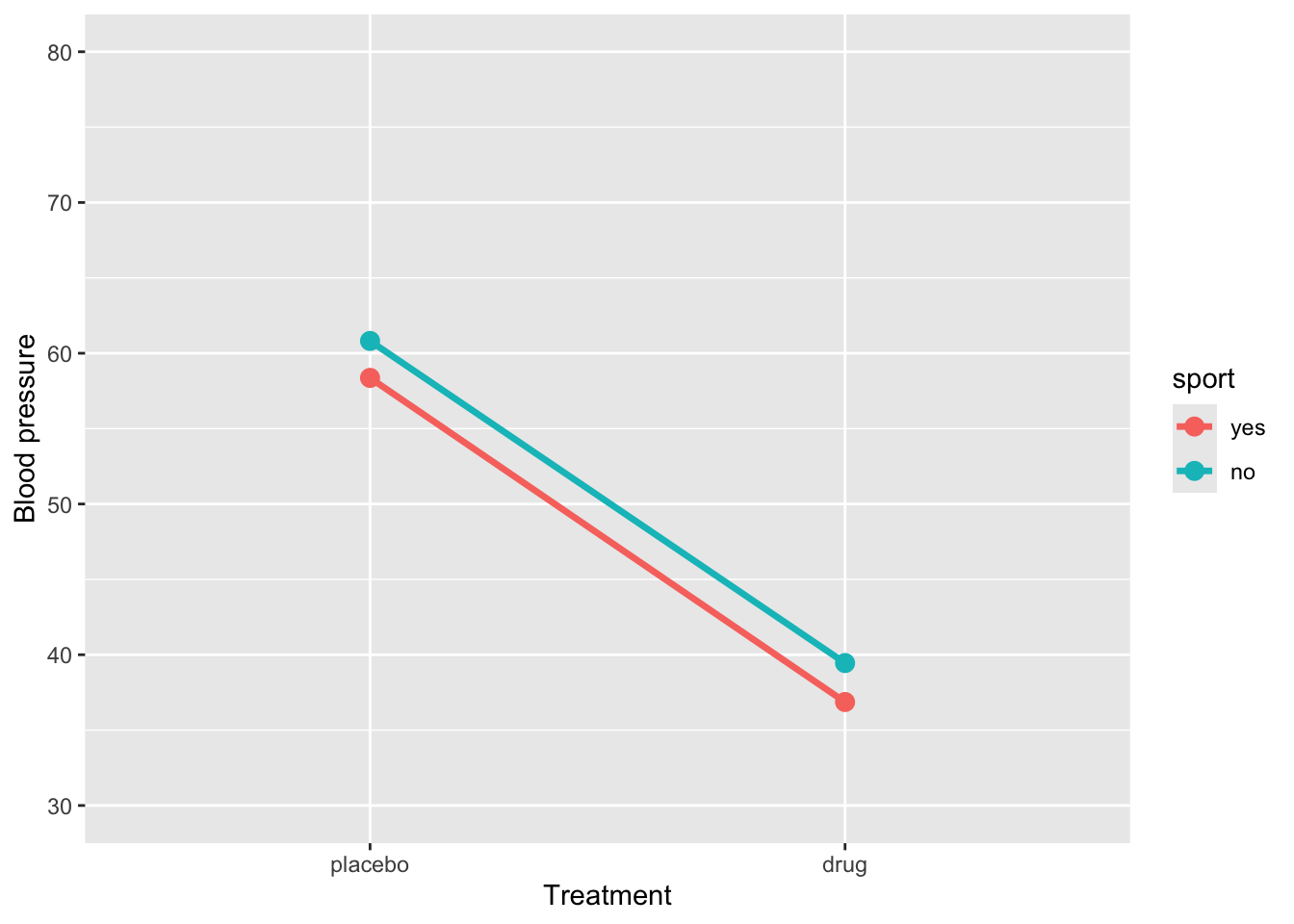
Fit the model with an interaction effect:
res1 <- lm(BP ~ treatment * sport, data = sim_data) |>
  tidy() |>
  mutate(
    p_value = as.numeric(formatC(p.value, format = "f", digits = 4)
  )) |>
  select(-p.value)

res1
# A tibble: 4 × 5
term estimate std.error statistic p_value
<chr> <dbl> <dbl> <dbl> <dbl>
1 (Intercept) 58.4 0.847 68.9 0
2 treatmentdrug -21.5 1.20 -18.0 0
3 sportno 2.45 1.20 2.05 0.043
4 treatmentdrug:sportno 0.135 1.69 0.0799 0.936The regression model shows that BP for the reference group (placebo and sport = yes) is 58.37. When sport = yes, taking the drug reduces BP by approximately -21.5units, a highly significant effect. Being in sport = no significantly increases BP (2.45) in the placebo group. The interaction between treatment and sport (0.14) indicates that the drug’s effect is slightly smaller for sport = no, but this difference is not statistically significant. Overall, the drug substantially reduces BP regardless of sport participation, and there is no meaningful interaction, so the effect of the drug is similar across both sport groups.
Example 2
# For reproducibility
set.seed(123)

# Define the design
design <- list(
  treatment = c("placebo", "drug"),
  sport = c("yes", "no")
)

# Define the means for each condition
mu <- c(38, 40, 38, 40)

# Simulate the data
sim_data2 <- sim_design(
  between = design,
  dv = "BP",
  mu = mu,
  n = 30,  # Number of participants per condition
  sd = 5,  # Standard deviation
  long = TRUE,
  plot = FALSE
)ggplot(sim_data2, aes(x = treatment, y = BP, group = sport, color = sport)) +
stat_summary(fun = mean, geom = "line", size = 1.2) +
stat_summary(fun = mean, geom = "point", size = 3) +
coord_cartesian(ylim = c(30, 50)) +
labs(y = "Mood", x = "Treatment")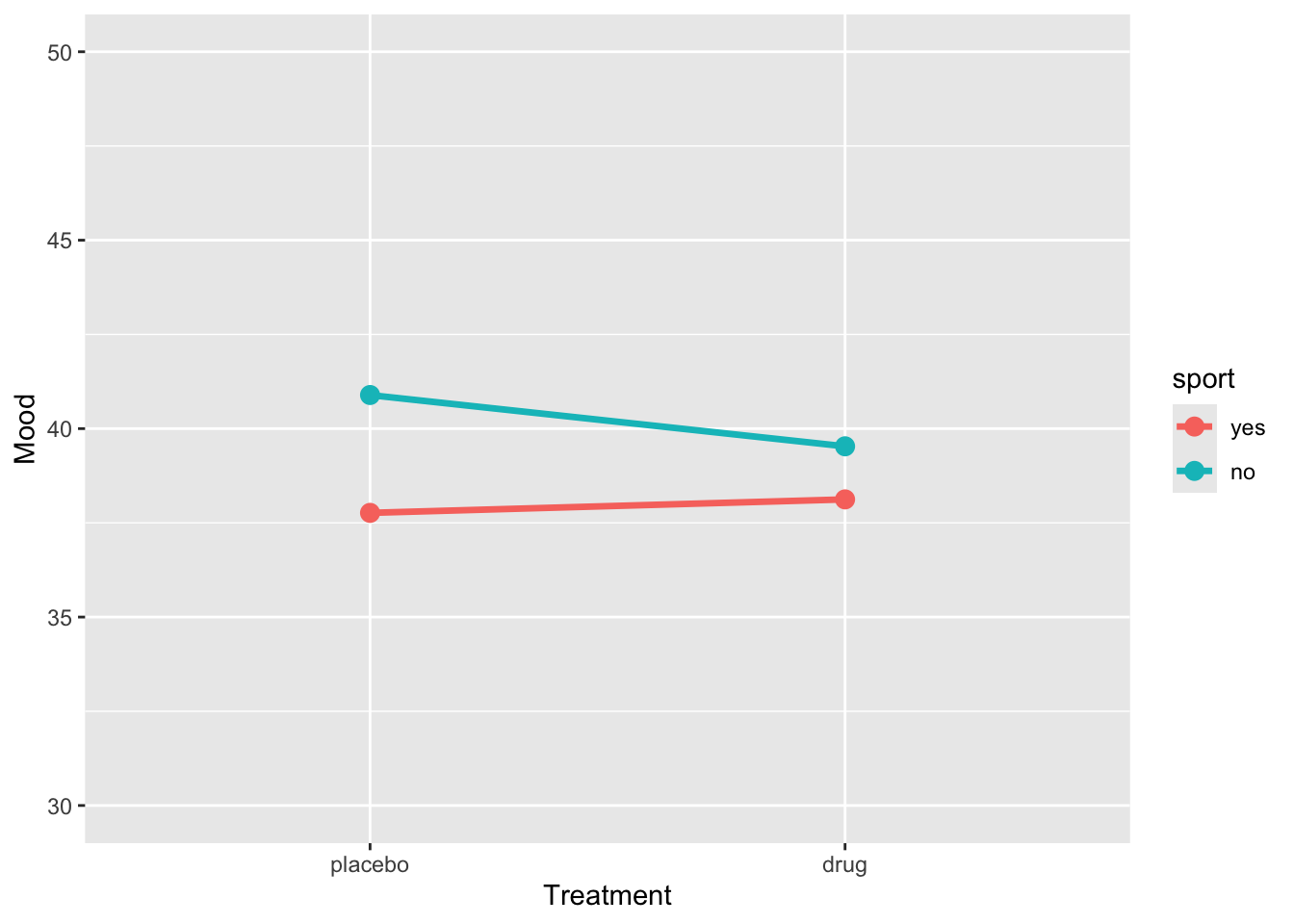
res2 <- lm(BP ~ treatment * sport, data = sim_data) |>
  tidy() |>
  mutate(
    p_value = as.numeric(formatC(p.value, format = "f", digits = 4)
  )) |>
  select(-p.value)

res2
# A tibble: 4 × 5
term estimate std.error statistic p_value
<chr> <dbl> <dbl> <dbl> <dbl>
1 (Intercept) 58.4 0.847 68.9 0
2 treatmentdrug -21.5 1.20 -18.0 0
3 sportno 2.45 1.20 2.05 0.043
4 treatmentdrug:sportno 0.135 1.69 0.0799 0.936Example 3
# For reproducibility
set.seed(123)

# Define the design
design <- list(
  treatment = c("placebo", "drug"),
  sport = c("yes", "no")
)

# Define the means for each condition
mu <- c(55, 62, 40, 55)

# Simulate the data
sim_data3 <- sim_design(
  between = design,
  dv = "BP",
  mu = mu,
  n = 30,  # Number of participants per condition
  sd = 5,  # Standard deviation
  long = TRUE,
  plot = FALSE
)
Let’s plot the data
ggplot(sim_data3, aes(x = treatment, y = BP, group = sport, color = sport)) +
  stat_summary(fun = mean, geom = "line", size = 1.2) +
  stat_summary(fun = mean, geom = "point", size = 3) +
  coord_cartesian(ylim = c(30, 80)) +
  labs(y = "Blood pressure", x = "Treatment")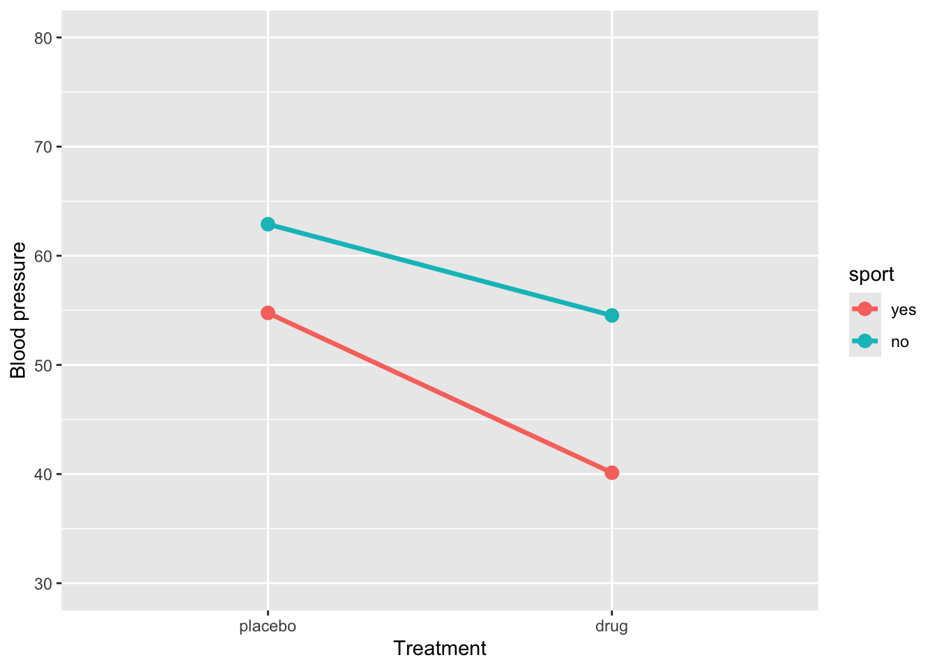
Let’s fit the model
# A tibble: 4 × 5
  term                  estimate std.error statistic  p.value
  <chr>                    <dbl>     <dbl>     <dbl>    <dbl>
1 (Intercept)              54.8      0.821     66.7  2.45e-94
2 treatmentdrug           -14.6      1.16     -12.6  1.80e-23
3 sportno                   8.13     1.16       7.00 1.81e-10
4 treatmentdrug:sportno     6.28     1.64       3.82 2.13e- 4
How to interpret this output:
(Intercept)= 54.8: This is the estimated mean blood pressure for subjects in the placebo group who are active.-
treatmentdrug= -14.6: This represents the change in blood pressure for subjects who are in the drug treatment and are active. Their blood pressure is:54.8 + -14.6 =
40.1
-
sportno= 8.1: This represents the change in blood pressure for subjects in placebo group and are sedentary. Their blood pressure is:54.8 + 8.1 =
62.9
-
treatmentdrug:sportno= 6.3: This is the interaction effect: the additional change in blood pressure for subjects who are sedentary and in the drug group. So, their expected blood pressure is:54.8 + (-14.6) + 8.1 + 6.3 =
54.5
An interaction effect occurs when the effect of one predictor varies depending on the level of another predictor. Graphically, this is shown when the lines representing different groups are not parallel. Conversely, parallel lines typically indicate the absence of an interaction, meaning the effect of one predictor is consistent across the levels of the other.
2.1.5 Interaction between a continuous and categorical predictors
Suppose we want to determine whether the effect of GPA on grade differs between students who play “team sports” and those who play “individual sports”. Specifically, we aim to compare whether the effect of GPA on grade varies as a function of sport.
ggplot(grades, aes(y = grade, x = GPA, colour = sport)) +
  geom_point() +
  geom_smooth(method = "lm", se = FALSE)
`geom_smooth()` using formula = 'y ~ x'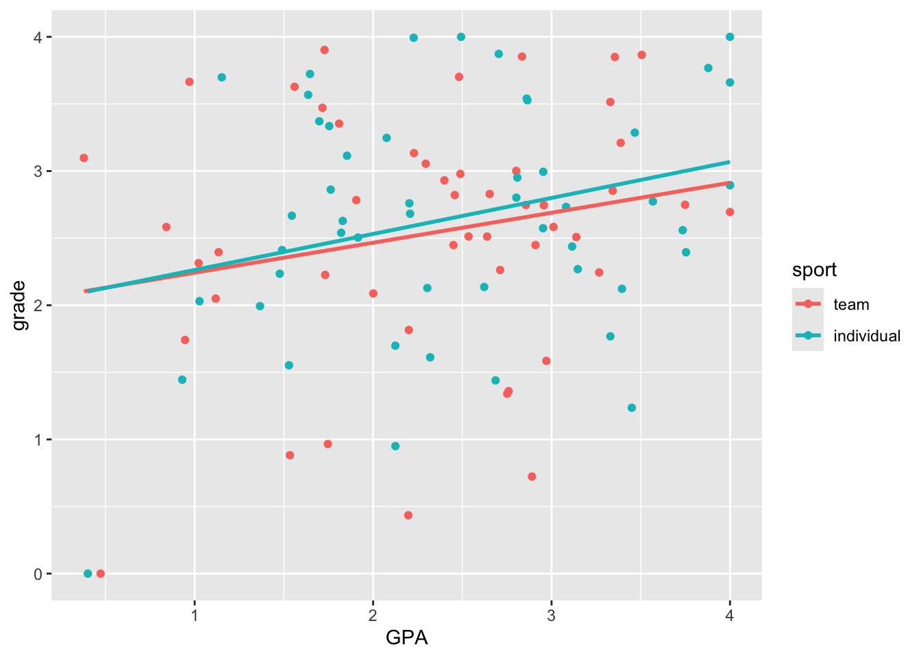
Here we see very clearly the difference in slope that we built into our data. How do we test whether the two slopes are significantly different? To do this, we can’t have two separate regressions. We need to bring the two regression lines into the same model. How do we do this?
lm(grade ~ GPA + sport + GPA*sport, grades) |>
  tidy() |>
  mutate(p.value = format.pval(p.value, digits = 3, scientific = FALSE)) |>
  kable() |>
kable_styling()| term | estimate | std.error | statistic | p.value |
|---|---|---|---|---|
| (Intercept) | 2.0187700 | 0.3520472 | 5.7343736 | 0.000000113 |
| GPA | 0.2234913 | 0.1394717 | 1.6024138 | 0.112 |
| sportindividual | -0.0241565 | 0.5034438 | -0.0479826 | 0.962 |
| GPA:sportindividual | 0.0448184 | 0.1965006 | 0.2280829 | 0.820 |